
THE GRAPHICAL LANGUAGE
Table of Contents
If you wish to improve immediately your practical know-ledge of MUSTIG operating system, please refer to the tutorial : you will be able to understand, through an example, both the calculating process and how the graphic editor works.
2-3 The dependence graph : basic graph
2-4 Compacting the graph into bundles
2. THE GRAPHICAL LANGUAGE
The language used by MUSTIG can be described from different points if view. The basic form is that of a dependence diagram completed by a syntax which allows a description of only one pattern from a periodic diagram by making up bundles, and rules allowing to condense the representation. Subsets of the graph may be compacted into "macros". As soon as a sufficient number of macros are present (those in the standard library for instance) it is possible to leave the basic form and pass to a functional form much closer to a mathematical description. The definition of the "delay" macro (z-1) allows the description of the filter structures in a flow diagram form. Finally, an analysis in a sequential form, more classical, is always possible and can be used especially for real-time applications.
All these forms are different approaches of the language. The calculation code made up by the compiler, starting from one form or the other will often be the same. Different forms may be mixed together in a unique analysis.
An analysis is made up by a graph which defines the connections between signals. These signals are functions of one or several discrete variables.
Examples:
f(t) temporal signal, function of the temporal variable "t"
f(x,y) spatial signal, function of two space variables "x" and "y"
f(x,y,t) spatio-temporal signal, function of both time and space variables.
It is most important to distinguish this notion of variable as a signal medium from that used in procedural programming languages where reference is made to a memory cell whose content may be changed. The notion aimed at in this manual is rather that from the mathematical vocabulary as a "function of a variable".
These (discrete) variables are given a name and their characteristics are as follows :
All these variables have a finite number of values (except, possibly, one : the time, in application of analysis in real-time). The definition of these variables is attached to the signal. For the techniques of definition of the variables, see section 4-3
A macro is a subset of the compacted graph represented by a box and could be as small as the boxes of the basic modules or quite large containing basic elements as well as other macros. It is identified by a name. This name may be followed, and separated by a "/" from them, by the name(s) of the variables used by the macro :

In the example above, the created macro module is named "My macro". The "/t/f/x" string entered after the name indicates that this macro processes three variables named t, f and x.
If the name of the variables is modified, the editor modifies all corresponding names inside the macro. Thus a macro operates on a variable named x for instance, and you now want it to process a signal carried by a variable named y, you just have to change the name by shift+ctrl+clicking on the variable names in front of the macro.

In fact, macros are used to conveniently reduce the dimension of the graph on the screen and make it easier to read. They change nothing in the compiler process, as the same calculations are run by the compiler.
Using macros allows for system and subsystem description as well as reduction of the space taken up by graph saving files since macros are saved only once, or not at all when they come from the basic library.
2-3 The dependence graph : basic graph
The analysis is described under a graph form which defines the relations of dependance (arithmetical, logical...) between the values (scalar or vector) ; this graph does not take into account the chronology of the generation process. All memories do not appear. This dependance graph must not include loops.
It is entered directly in its graphic form and is made from elementary mathematical operators (see figure below for example). These operators are drawn as rectangles, with "pins" where "wires" of propagating values are "connected". The operators are identified by a name or a symbol within the rectangle.
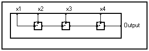
Some operators operate on scalars, others on vectors, therefore the variable (s) must be entered after the name separated by the "/" (slash) sign.
2-4 Compacting the graph into bundles
In many applications, some inputs and outputs of the diagram are vectors and the diagram has repeated structures which are represented in a mathematical language by recurrent equations. The graph can be compactly represented as a bundle. Only one pattern is drawn from the periodical structure of the graph, and placed within a rectangle with a thicker edge in the direction where the pattern should be repeated to obtain the whole graph (see figure below).
By convention, the thicker edge is placed in the direction of increasing indices. The thicker line represents in a schematic way the thickness of the bundle. This compacted set will be called a bundle (if we think of how it was made up) or a "looping" if we think of its equivalent in classical programming languages.
To get a better understanting of this notion, imagine that all the identical patterns of the graph have been drawn on cardboard rectangles, then have all been gathered into a bundle, just like playing cards.

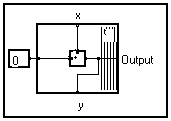

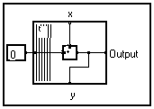
A pin placed on the thicker edge has necessarily a corresponding pin on the facing edge. An output always corresponds to an input and reciprocally. This is an immediate consequence of the way the bundle is constituted : when patterns were side by side, an output was directly linked to an input of the adjacent pattern. These pins are called "frontal pins".
On both other sides, can be found (or not) pins which are called "lateral pins". The link connected to a lateral pin corresponds to the unique representation of the set of links to each original pattern. We suppose that all the links of the initial graph were scalar values ; then the set of scalars forms a vector-value. To be more precise, we will write that it is a function of the variable used as an index in patterns and is indicated in the thicker edge of the bundle.
Note :
As the edge of the bundle is drawn in a thicker line, it would be logical to do the same when drawing lateral links, this would show their vector-valued characteristic, but this would make the graph too heavy.Compacting into bundles can be repeated if the initial diagram presents a double frequency. Now, the values of the frontal inputs are not scalar : lateral outputs become functions of the same variables as the frontal inputs and of the bundle variable.
The same could be applied to lateral inputs, except that the expanding mechanism allows the signal not to be function of the bundle variable.
The graph layout is made easier by using the following vector function modes, two simplifying properties of MUSTIG.
If a vector-valued signal is applied to a scalar operator, all the elements of the vector are affected by the operation. More generally, if a signal depending on more variables than the operator knows is applied to this operator, the operation is carried out on each element taking into account the additional variable(s).

If both a vector and a scalar are applied to a scalar operator, the operation is carried out onto each element on the vector with the same scalar value. For example, if the addition operator is applied to a scalar and a vector, the scalar will be added to each element of the vector : the output is therefore a vector.
More generally, if two signals are applied to an operator with one of them depending on one variable less than the other, the operator becomes a function of this variable, but its value is a constant along this variable.

In the case of a vector-valued operator, signals must be a function of the variables expected by the operator.
Implicit repetition reduces the graph by taking out some operators from the bundles. Thus, lateral edges of the bundles are permeable boundaries : operators can pass through them ; when continuity of the connections is maintained nothing is changed in the graph significance.
|
|
<=> |
|
This rule allows to apply to multidimensional signal any analysis planned for single dimension signals. These two rules, combined with the possibility of compacting parts of the graph into macros acting as new operators, allows many analysis problems to be described entirely in the form of a functional diagram, without calling the basic form of the dependence diagram.
Analysis systems such as filters are often described by flow diagrams. This diagram is a direct transcription of the difference equations of the filter, using arithmetical operators and elementary delays.
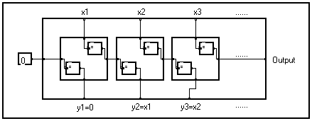
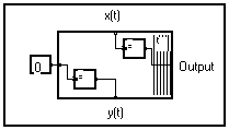
These delays, whose transfer function in z is "z-1" can be easily built through the basic syntax. One must only draw the dependence diagram which links the input samples to the output samples of the delay. This diagram has no operator, it only has links. The compacted form in bundles is deduced and the macro form designed to get the delay operator.
Please note that it is possible to apply this operator to a signal depending on several variables, the delay is executed along the variable indicated in the bundle and found on the macro.
In fact the graphic editor forbids the building of a bundle without an operator, thus the ineffective operators "=" is introduced.
![]()
The first sample of the delayed signal does not depend on the input signal. Its value, given by the frontal input of the bundle, is set to 0 in the macro of the standard library but it can be altered.
Reasoning in discrete temporal system simulation, this first value corresponds to the initial state of the memory cell. If needed, this value can be accessed through an additional entry of the macro. In the same way, the last value of the input can be taken out, otherwise it is normally lost. A generalized cell is obtained with four pins as shown above.
A flow diagram may have loops. This may seem contradictory with the fact that loops are not permitted in the dependance graph. In fact, when replacing "z-1" macros by their content, a graph with no loops is obtained and the calculation is possible.
The indefinite integral y(t) of a signal x(t) of the discrete variable t can be calculated through the recurrent relation :
y(t) = x(t)+y(t-1) with y(0) = x(0) for t = 0
This relation can be expressed by the flow diagram shown below :
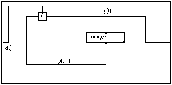
Expanding the delay/t macro, we obtain :
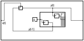
We have seen that lateral boundaries of a bundle may be crossed without changing the signification of the graph. Thus the adder may be added to the bundle :
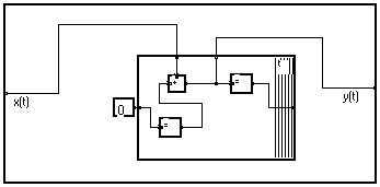
The graph can be further simplified, giving the same diagram obtained when starting from the dependence diagram :
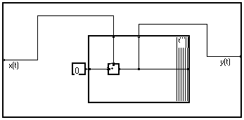
Practically, the compact form in macro "Sum/t" will be much easier to read :
![]()