4-8-1. Characteristics of MUSTIG variables
As seen in chapter 2, each wire of the graph carries a signal which, in the most frequent case where it is not a single scalar, depends on one or several variables. The name of the variable processed by a module or a macro is indicated on its front panel. It can be edited and changed using Shift+Ctrl+Click in order to process another variable.
4-8-1. Characteristics of MUSTIG variables
Each variable (also called a dimension) is defined by seven parameters or attributes, which may be individually changed using modules from the Variable changes section of the Library :
|
Name |
Appears in the Value input module or on the front panel of macros and modules right after the '/' sign. Ex. : /t denotes a variable named t (default name for many modules). The name of a variable may be edited and changed (Shift+Ctrl+Click). |
|
Length |
Number of samples of the signal along the dimension (no default, must be explicitly set by the user). Reminder : the index of the first sample along a dimension is 0, not 1. A particular value is -1 : the number of samples is infinite and the simulations will be carried out until the user clicks again in the Mustig window to stop it. Be aware not to use viewing modules intended for finite signals to view infinite signals, for the simulation could not be stopped ! Use modules from the Outputs / real time section of the Library instead. |
|
Origin |
Actual date of the first sample (index=0). The default value is 0. |
|
Pitch |
Sampling rate T in seconds (default value is 1 s), i.e. time gap between two consecutive samples. T=1/Fe where Fe is the sampling frequency. When a Fourier Transform is carried out, the characteristics of the generated frequency variable are set according to the sampling rate, so that the frequency domain spreads from 0 Hz to Fe/2 Hz. |
|
Dual |
Default value is 0. Changed into 1 if a Fourier Transform is carried out on the signal. |
|
Half |
Default value is 0. Changed to 1 if the signal is made of the first N/2+1 points from a N samples complex signal with Hermitian symmetry (for example if the signal is issued from the Fourier transform of a real signal). |
|
Dual Origin |
Sets the origin of the variable in the frequency domain for a time-domain signal, and conversely. Default value is 0. |
CAUTION : Variable indices begin at index 0 like in C language.
The Attributes which have no default value (i.e. name and length of the dimension) must be defined when starting a new branch of the Mustig graph (see Defining a variable).
If a module requires at least two input signals, and if each of these signals depend on a variable with the same name, the characteristics of the two variables must be identical.
Variables may be explicitly defined by the user, or automatically derived from the characteristics of another variable in the graph.
Defining a variable from the Value scalar input module
Although the Value module in the Inputs section of the Library is intended to entering scalar values, it may be used to conveniently define small vectors.
In order to do this, just enter the successive samples along the dimension you want to create, separating them by a carriage return, then enter the name you wish to give this new dimension on the last line, right after a '/' sign :

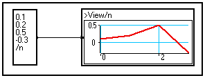
In the above example, a vector is defined : it contains four elements and the created variable is named n. The default sampling rate is 1 second, the default origin is 0 as seen on the graph.
N.B. : This vector is viewed using the standard View/t module : we have just edited and changed the name of the variable to process on its front panel (Shift+Ctrl+Click), moved the graphical window onto the front panel for convenience (see Creating images), and changed the default line into a thick red line.
Defining a variable using the variable definition modules
You may create a variable carrying any number of samples by using any of the two following modules :
|
|
Creates a dimension according to a variable named t and containing 256 samples. The name and the number of samples may be edited and changed (Shift+Ctrl+Click). |
|
|
Does exactly the same : the N/t module creates a variable named t containing the number of samples on the input pin. This allows to create a variable from a number of samples derived from a calculation. |
|
|
Allows to create a variable named t. All the attributes (number of samples, origin, sample rate, etc) are set by double-clicking on the box :
|
Using a previously defined variable
Any wire in the MUSTIG graph contains the whole information about the variables it carries. Thus, it is possible to create a variable having the same characteristics than a previously defined one by simply plugging a wire at a location where the information is present.
This technique may be used to build several signals from the same variable. You are thus sure you can add, multiply, etc. the signals, for they have exactly the same characteristics.
Example : Suppose you want to add a noise and a sine wave. You could build the two signals separately like in the graph below :

However, if you change any characteristic of a signal (e.g. the sampling rate), you will have to perform the same changes on the other signal, otherwise you mill not be able to add them.
Thus, it is much more efficient to directly pick up all the information about variable t from a wire to build the signals :
 or
or 
You may also pick up the information about a variable and change a few characteristics before using it :

In the above example, two signals containing 100 samples each with a default 1Hz sampling frequency are created. A sine wave is built on this variable t (top). In the bottom branch of the graph the sampling rate is changed into 100Hz before building the sine wave with the same number of samples.
A variable is said to be dynamic when the length of the signal along this variable depends on another variable. Dynamic variables can be defined by entering a vector of lengths in a Part or Part_shift module (see Changing the attributes of a variable dynamically).
They may also be directly defined using the Var_dyna/t module in the Variable changes section of the Library :
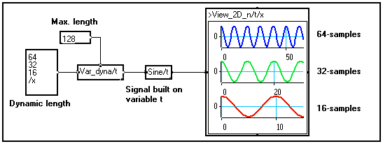
In the above example a dynamic variable named t is created : its length depends on another variable named x. After the Var_dyna/t module, a sine wave of frequency 0.1Hz is built on the created dynamic variable. The sine wave is thus generated three times : one sine wave with 64 samples, one with only 32 samples and one with 16 samples.
Note that the View_2D_n/t/x two-dimensional viewing module allows to view signals carried by dynamic variables (the length of the three displayed signals is different). In the above example, the graphical window has been slid into the front panel of the viewing module in order to create a preview module (see Creating an image). The Individual composite lines option has been set to change the look of the curves individually.
4-8-3. Changing the attributes of a variable
Specific modules allow to change the characteristics of a variable (or dimension) individually. They are located in the Variable changes section of the Library.
Changing the name of a variable
The ChVar/u/v module in the Variable changes section of the Library allows to change the name of a variable from u into v. You may of course edit and change the old and new names of the variables.
In the example below a 100 samples variable named t is generated and a sine wave is built from this variable. The name of the variable is changed into tau before building another sine wave according to variable tau. Except their name, both variables have the same characteristics.

Changing the sampling rate of a signal
When a variable is created, the default sampling rate is 1Hz (supposing this variable denotes the time). When may want to change it in order your simulations to be closer to reality. You can do this using the Pitch/t module in the Variable changes section of the Library :
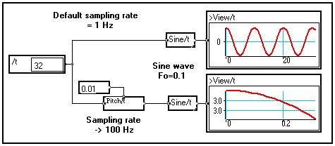
The input value on the top pin of the Pitch module is the new sampling rate of the signal, that is, the gap (in seconds if variable /t is time) between two consecutive samples.
The frequency of the sine wave is in Hertz, so that the result depends on the sampling frequency Fe of the signal : in the top case the frequency of the sine wave is Fe/10, in the bottom case it is only Fe/1000.
Note that the View/t macro displays dates along its horizontal axis, not indices.
Changing the origin of a signal
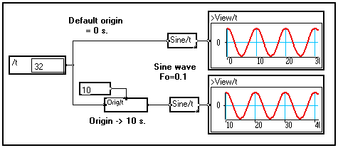
The origin of a signal is the date (in seconds if variable /t is time) associated with the first sample of the signal. It may be changed using the Origin module in the Variable changes section of the Library :
Changing the length of a variable
Several modules exist to change the number of samples according to a dimension. They allow to select a part of a signal, or increase its length by zero-padding. Check their online help for more information on how to use them.
|
|
Extracts a given number of consecutive samples, starting at a given position (in samples). The origin of the extracted vector is modified accordingly. If the number of samples to extracts is larger than the number of available samples in the signal, zeros are generated to fill the space. |
|
|
Same as above, but the origin of the vector is unchanged |
|
|
Same as the first one, but the position (in samples) of the first and last samples to extract are set by double-clicking on the box. |
|
|
Same as above, but the position of the first and last samples to extract are expressed in seconds (is the processed variable is time) instead of in samples. That is, the position in samples is derived from the sample rate and origin of the variable. |
Changing the attributes of a variable dynamically
The attributes of a variable are generally static : they cannot depend on another variable.
In the example below, a three-element vector depending on variable /x is added to a four-element vector depending on variable /t.
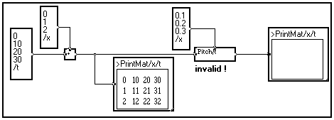
This operation is valid because the signals have different variable names : the output of the adder is thus a matrix depending on variables /t and /x. The latter can be viewed as a set of three vectors depending on variable /t, the indices of variable /x denoting the rank of a vector : 0, 1 or 2.
Then, we try to define a different sampling rate for each of the three vector by using the Pitch module with three values depending on variable /x : one for each of the three vectors.
Although this graph is consistent, the Pitch module will not accept a non-scalar input on its top pin, as the sampling rate of a signal cannot depend on another variable. If you try to display the matrix after the Pitch module you will get the following error message : The variable definitions must be static.
An exception to this is the length of a vector : in some cases it may be dynamic. That is, the length of a vector may depend on another variable. As a matter of fact, the Part and Part_shift modules accept both scalar and vectorial inputs :
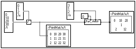
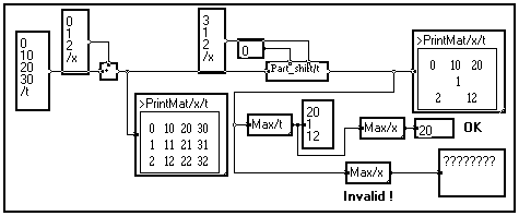
In the above example, the Part_shift module cuts vectors of variable length (3,1 and 2 elements) from the rows of the input 3x4 matrix. This output of the module is thus a dynamic set of vector : the length of a vector depending on variable /t depends on its rank according to variable /x.
Remarks on dynamic changes of the length of a signal
You may change the dual attributes of a signal if necessary (see Variable attributes to know what Dual attributes are used for) :
|
|
Sets the Dual attribute of a variable to the value entered on the top pin. |
|
|
Sets the Half attribute of a variable to the value entered on the top pin. |
However this is rarely done explicitly, for the information about a variable created by a Fourier Transform can generally be picked up directly.
Example : Suppose you want to create a rough low-pass filter by selecting only the low frequency Fourier coefficients of a signal. Instead of creating the filter template separately like in the graph below :

It is much more clever to extract the information about the frequency variable f from a wire after the Fourier Transform. You don't have to bother calculating the frequency pitch and setting the Dual and Half attributes to one : all the attributes are set to their correct value by the Fourier Transform.
The correct graph is more compact, more general, and easier to understand :

Therefore, by connecting to appropriate wires on the graph, you will generally be able to avoid explicitly changing the dual attributes of a signal.
Additional modules are available in the Variable changes section of the Library to perform basic operations on variables, such as :
Check out the online help of the described modules for more information on how they operate and how to connect their pins.
Undersampling and oversampling a signal
Modules are available in the Variable changes section of the Library to perform under- or over-sampling of a signal. Check out their online help to know how they should be used.
|
|
Under-samples a signal. The under-sampling factor is entered on the top pin. This module requires the whole input signal to be memorized. |
|
|
Asynchronous undersampling : samples a vector according to a "logical" conditioning vector. |
|
|
Asynchronous sampling with regular spacing. |
|
|
Oversamples a signal by a given factor, inserting zeros |
|
|
Sample and Hold oversampling |
|
|
Oversampling with linear interpolation between samples. |
Extracting a value from a vector
Modules are available in the Variable changes section of the Library to extract a given sample from a vector. Check out their online help to know how they should be used. Reminder : In MUSTIG like in C, the first element of a vector is referred to by index 0, not 1.
|
|
Extracts the first element according to variable u. The name of the variable may be edited and changed (Shift+Ctrl+Click). |
|
|
Extracts the last element according to variable u. The name of the variable may be edited and changed (Shift+Ctrl+Click). |
|
|
Extracts the element located at the index entered on the top pin (in samples). |
|
|
Same as above except that the index of the extracted sample is set by double-clicking on the box. |
If the cutting index entered on the top pin is larger than the signal length, the output result is zero.
As a single value is extracted from the dimension entered on the front panel (e.g. /u on the modules above), the output data does not depend on this variable any more. If the input data depend on two variables or more, and a "Cut" operation is carried out according to one dimension, the cutting operation is carried out for every occurrence of the other dimensions.
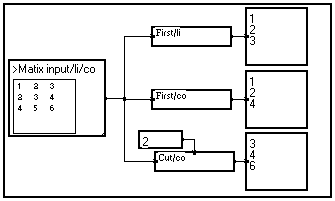
Example : Extraction of a column or a line from a matrix.
Here, the input signal is a matrix. If you cut a sample according to the lines (variable /li) you obtain a line of the matrix (according to variable /co), for the cutting operation has been carried out on every column.
On the other hand, if you cut according to variable /co, the cutting operation is carried out on every line of the matrix and you obtain a vector equal to a particular column of the matrix.
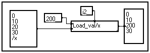
In some cases you may need to change the value in a vector at a given index. You can do this directly using the Load_val/t macro in the Variable changes section of the Library. In the example below, the value of the third element of the vector (index = 2) is changed into 200 :
Converting indices into dates, or dates into indices
When a variable is defined, a given sample index no is associated to a given date to in seconds, which depends on the origin and the sampling rate D t (both in seconds) set by the user (see Changing the sampling rate of a variable) :
![]()
When you perform operations such as extracting a value from a vector, selecting a portion of a vector, etc., in some cases you must enter the indices of the sample(s) to select, and in some other cases you must enter their dates.
The I->V/t and V->I/t macros in the Variable changes section of the Library allow to respectively derive dates from indices, and indices from dates :

Splitting a signal into a cluster of sub-signals
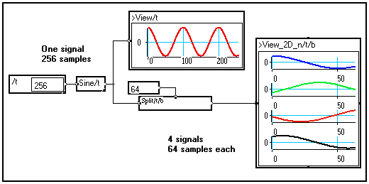
For some applications it is necessary to split a signal into several shorter parts. This can be done automatically by using the Split/t/b module in the Variable changes section of the Library :
Merging a cluster of sub-signals into a single signal
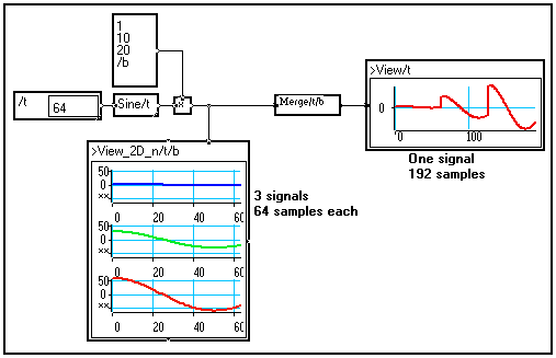
A two-dimensional cluster of signals can be merged into a single, longer signal by using the Merge/t/b module available in the Variable changes section of the Library :
Demultiplexing a signal into several sub-signals
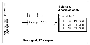
You may split a signal into several sub-signals, assuming that the original signal was produced by a multiplexer. The demultiplex/t/p module is available in the Variable changes section of the Library. The module creates a new variable (/p in the example below) which can be considered as the channel number after the demultiplexing operation :
Multiplexing signals into a single signal
You may merge a group of signal into a single one as it is done by a multiplexer. The Multiplex/t/p module is available in the Variable changes section of the Library :
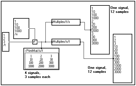
After the multiplexing operation, the signal depends on only one variable. As shown on the above example, the order in which the samples are merged depends on the order of the variables (/x/t or /t/x) set by the user in the front panel of the Multiplex module.
The Concatenate/t macro in the Variable changes / Operations on vectors section of the Library allows to concatenate two signals depending on the same variable.

In the above example a 100-sample 5Hz sine wave is concatenated to a 150-sample 1Hz sine wave. The result is a 250-sample (=2.5 seconds here) signal.
Both signals must have the same variable name and the same attributes, except that their length may be different.
Expanding the dimension of a signal
You may expand the dimension of the signal, that is, create a vector from a scalar, a matrix from a vector, a 3D tensor from a matrix, and so on, by using the "=" module in the Variable changes section of the Library :

Getting general information about the signals carried by a wire
A very useful macro is the Info macro in the Variable changes section of the Library. When connected to a wire, this final box provides the user with general information on the signals carried by the wire : type of data, name, length, origin, etc. of the variables :

If you calculate the Info macro by right-clicking on it, a new window opens :

It indicates that this wire contains 4-byte real data (R4), described by two variables /t (length 256 samples, sampling rate 100Hz, origin 10s) and /gain (length 4, default sampling rate 1Hz). This group of data can thus be viewed either as a 4x256 matrix, or as a cluster of 4 signals containing 256 samples each.
If the length is displayed in brackets, the corresponding variable is a dynamic variable : its length depends on another variable. The displayed length is the maximum length of the variable.
4-8-4. Transmitting the variable information to a bundle box.
Bundle boxes are used to build algorithms that process the elements of a vector individually, instead of carrying out the same operations on all the samples of a vector. Although a large number of operations is proposed in the Library, you may have to build bundles by yourself if this is required by your application.
See : Compacting the graph into bundles or loops
Creating bundle boxes
As a bundle is a process that refers to a variable, the user must provide the bundle with information about the variable it must process. This variable may be an existing variable, or it may be created on purpose.
Looping on an existing variable
If a signal is not a scalar, it carries information about its variables. If such a signal comes on a lateral pin of a bundle box, and if the signal depends on the variable of the bundle box, the information required to the loop calculations are known.
For instance, let a signal be a function of variable t and let us calculate the sum of the elements of this signal along t. The MUSTIG program will be :
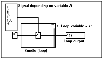
The loop variable is the same than that carried out by the incoming signal. This variable is named /t and carries a five-sample signal. Thus, the bundle performs five loops, one for each sample of the input signal, and gives the sum of the elements as a result.
Therefore, when the variable on which you want to loop already exists, the graph is quite simple to build.
If the loop variable is not carried by one of its input signals, a specific variable must be created and connected to a lateral pin on the border of the bundle.
In order to do that, just define the loop variable outside the bundle box (see Creating a variable), and create a wire between the output of this variable definition and a lateral pin of the bundle box, not already linked (see Creating a pin).
Suppose for instance you want to generate a vector made of successive powers of a given number : X={1,a,a2,a3,...,aN-1}, where a is a scalar. A good way of doing this is to start with a "seed" (a=3 for instance), and multiply it by itself a given number N of times.
This can easily be done with a bundle like in the program below (for a = 3 and N = 5) :
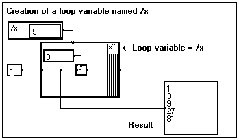
As you start with a scalar seed (a), no variable is available for looping. However, you must tell the bundle how many times it should loop ! This is done by creating the new variable /x and connecting it to a lateral pin created on the border of the bundle.
This variable /x has been defined but it does not contain any value, it is not an actual "signal". All the bundle needs here is its length, in order to know how many loops should be carried out. This is why connecting the lateral pin to a calculation module inside the loop is not required.
The obtained result is taken from inside the loop. It is thus a vector depending on the loop variable /x. It contains five samples, which corresponds to the values carried by the wire at each of the five iterations of the loop (see Compacting the graph into bundles or loops).