Recursive filtering
Content
Realization of filters defined by a difference equation by a flux diagram. Filters of the first order, cells of the second order, cascade of cells of the second order. Use on a continuation of blocks.
Key words
filtering, flux diagram ,calculation by blocks
MUSTIG Files
Related commented examples
transverse filtering, filtering by DFT
Theoretical principles
In a general way, a linear discrete filter can be defined by a finite differences
equation binding the input of the filter ![]() and its output
and its output![]() .
.
![]()
In the particular case where all coefficients ![]() (for
(for
![]() ) are null, the impulse answer of the filter
) are null, the impulse answer of the filter
![]() is of finished length and
is of finished length and
![]() . One then qualifies the filter of Finished Impulse Response filter
(FIR).
. One then qualifies the filter of Finished Impulse Response filter
(FIR).
In the other cases, one qualifies it of Infinite Impulse Response filter (IIR). The sample of the output signal of rank n being a function of the previous samples (of ranks n-1, n-2...) of the same signal, one often qualifies this type of filter as "recursive filter ".
One can replace the writing of the differences equation by a graph composed of operators " adder ", " gain " and " delay ". One calls this graph a " flux diagram ". This graph can serve to the physical implementation of the filter.
By transformation in " Z " of the differences equation , one builds the transfer function of the
filter, which is the " Z " transform of the impulse response of the filter
![]() . The factorisation of this transfer function puts in evidence
its poles and zeros, that can inform notably on the stability of the filter.
This factorisation allows to put the expression of the transfer function under the shape of a product of terms of order two.
Each of them correspond to a filter of order two, of which the difference equation will
be :
. The factorisation of this transfer function puts in evidence
its poles and zeros, that can inform notably on the stability of the filter.
This factorisation allows to put the expression of the transfer function under the shape of a product of terms of order two.
Each of them correspond to a filter of order two, of which the difference equation will
be :
![]()
or a normalized shape with ![]() and
and ![]() :
:
![]()
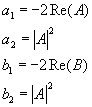
If this filter has real coefficients, its poles and zeros are complex conjugated.
While noting ![]() one of the
poles and
one of the
poles and ![]() one of the zeros, the coefficients of the cell of the second order
are :
one of the zeros, the coefficients of the cell of the second order
are :
MUSTIG realization
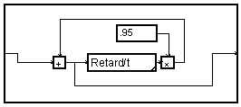
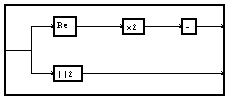
Recursive filter of the first order
The finite differences equation the simplest of this filter, writes :
![]()
One can calculate this equation by an iteration:
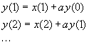
This iteration is achieved by the MUSTIG graph:
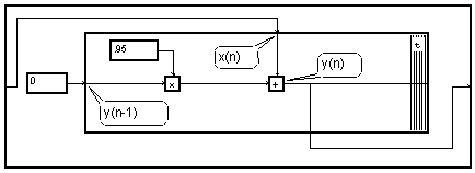
Let's note that ![]() is
initialized previously to a value arbitrarily fixed to zero.
is
initialized previously to a value arbitrarily fixed to zero.
This shape of graph, simple for a filter of the first order, would become very heavy for a large order. It will be generally easier to use a graph of type "flux diagram".
Under this shape, the initial value, ![]() is not visible, because it is the initial value of the " delay ".
It is possible to modify this macro to change this initial value.
In some cases, it will be also necessary to modify the type of this initial value.
is not visible, because it is the initial value of the " delay ".
It is possible to modify this macro to change this initial value.
In some cases, it will be also necessary to modify the type of this initial value.
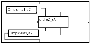
Let's note that the two previous shapes of filter are completely equivalent for the MUSTIG compiler that will generate the same code of calculation precisely in the two cases (See paragraph 2-6 of the manual for more precise explanations).
Filter of the second order
One uses one of the shapes of flux diagram of the cell of filter of order two, with the coefficient,
![]() . Its MUSTIG realization comes back to the simple drawing of this diagram of flux.
. Its MUSTIG realization comes back to the simple drawing of this diagram of flux.
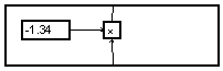
One can facilitate the drawing of such diagrams with fix coefficients is using a macro " gain ":
![]()
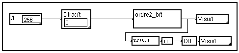
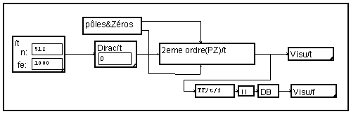
To verify the working of this filter, one can observe its impulse response while injecting it a " dirac ". The Fourier Transform of its impulse response gives the frequency response.
Filter of the second order defined by its poles and zeros
If one prefers to define the filter by the values (complex) of its poles and zeros, one adds the macro
which calculates the coefficients a or b from the zeros or poles
We use the macro " poles and zeros " to graphically define their position in the complex plane
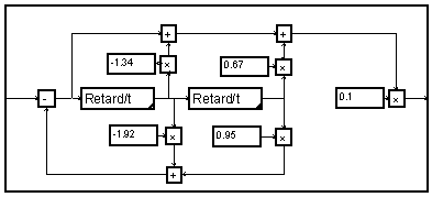
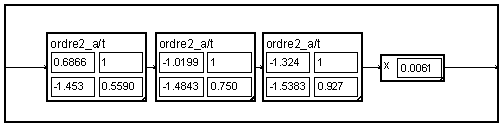
Cascade of filter cells of the second order
To achieve a cascade of filters, one can place several macros " ordre_2 " in cascade. It will be then convenient to put the coefficients in image on the macro to be able to edit them easily.
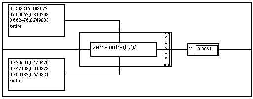
One can avoid the duplication of the cells and can only draw one motif of it in a " bundle ". For it, we will need to replace the scalar coefficients by functions of the bundle variable. It is simpler for it to use the macro " 2eme ordre(PZ) " whose entries are the complex values of one of the conjugated poles and of one of the conjugated zeros . One forms a list of values of poles function of the variable " order ". One makes in the same way for the zeros.
Recursive filtering of a suite of blocks
To apply a recursive filter on a long signal recorded on a disk file, it would be possible to read and to write the values one by one (See examples " reading files "). It may to be too slow. On the other hand, one can need to achieve spectral analysis, working on blocks, together with recursive filtering.
If one applies without modification a signal cut into blocks to a recursive filter, each of the blocks is going to be filtered independently of the other with a filter reset at the beginning of every block. To get a continuous filtering, one needs taht the initial state of the filter of a block be the final state of the filter of the previous block. In the form flux diagram, the state of the filter is contained in the delays. it is sufficient therefore to loop the final state of a delay on its input with the help of a bundle MUSTIG indexed by the variable of the blocks. It is made by replacing in the filter all " Delay/t " by the macro " Delay/t/b ".